PyTorch Workflow

This mainly covers the typical workflow of a PyTorch Model. That is, how we:

How we gather and prepare the data
How do we build the model, consisting of a. How do we evaluate our model (loss function design) b. How do we train our model (backprop and whatnot, aka training loop)
Run the model training
Evaluate the model
Make changes to hyperparameters
Ship model (save and reload, there’s also downstream shipping for deployment)

import torch 
from torch import nn
import matplotlib.pyplot as plt
 
torch.__version__
 
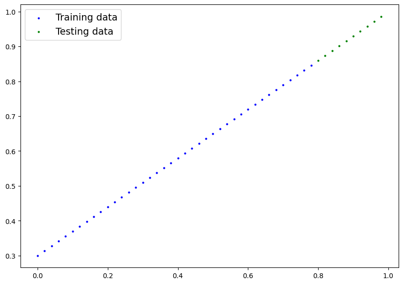
# Create a sample dataset representing a straight line
weight = 0.7
bias = 0.3
 
start = 0
end = 1
step = 0.02
X = torch.arange(start, end, step).unsqueeze(dim=1)
y = weight * X + bias
 
print(X[:10], y[:10])
 
# Split data into training and test sets
split = 0.8
split_i = int(split * len(X))
X_train, y_train = X[:split_i], y[:split_i]
X_test, y_test = X[split_i:], y[split_i:]
 
len(X_train), len(X_test)
 
# Plot
def plot_predictions(train_data=X_train, 
                     train_labels=y_train, 
                     test_data=X_test, 
                     test_labels=y_test, 
                     predictions=None):
  """
  Plots training data, test data and compares predictions.
  """
  plt.figure(figsize=(10, 7))
 
  # Plot training data in blue
  plt.scatter(train_data, train_labels, c="b", s=4, label="Training data")
  
  # Plot test data in green
  plt.scatter(test_data, test_labels, c="g", s=4, label="Testing data")
 
  if predictions is not None:
    # Plot the predictions in red (predictions were made on the test data)
    plt.scatter(test_data, predictions, c="r", s=4, label="Predictions")
 
  # Show the legend
  plt.legend(prop={"size": 14})
 
plot_predictions()

Output:

tensor([[0.0000],
        [0.0200],
        [0.0400],
        [0.0600],
        [0.0800],
        [0.1000],
        [0.1200],
        [0.1400],
        [0.1600],
        [0.1800]]) tensor([[0.3000],
        [0.3140],
        [0.3280],
        [0.3420],
        [0.3560],
        [0.3700],
        [0.3840],
        [0.3980],
        [0.4120],
        [0.4260]])

Output:

<Figure size 1000x700 with 1 Axes>

# Build the model
class LinearRegressionModel(nn.Module):
  def __init__(self):
    super().__init__()
    
    # initialize the weight as a random float value
    # requires_grad <> does this value get updated with backprop?
    self.weights = nn.Parameter(torch.randn(1, dtype=torch.float), requires_grad=True)
 
    # initialize bias as a random float value
    self.bias = nn.Parameter(torch.randn(1, dtype=torch.float), requires_grad=True)
 
  # forward is a function that needs to be implemented for an nn.Module
  # it defines the forward propagation of the model
  def forward(self, x: torch.Tensor) -> torch.Tensor:
    return self.weights * x + self.bias

PyTorch Model Workflow Essentials

They are torch.nn for the model itself, torch.optim which contains a bunch of optimization algorithms, torch.utils.data.Dataset that defines the dataset, and torch.utils.data.DataLoader to help with loading data into the model.

Torch.nn

torch.nn contains the modules to build computational graphs
torch.nn.Parameter stores tensors as parameters to be used in the nn.Module. If requires_grad is True, then gradients are automatically calculated.
torch.nn.Module defines the base class for all PyTorch neural network modules. Requires forward() to be implemented.
torch.optim contains a bunch of optimization algorithms for parameter optimization.
def forward(): all nn.Module subclasses must implement this.

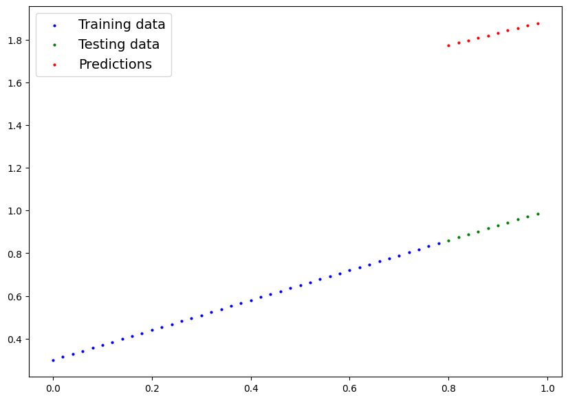
# Checking the current state of the model.
torch.manual_seed(88)
 
model = LinearRegressionModel()
list(model.parameters()), model.state_dict()
 
# this tells the model to not do any gradient descent, 
# disables a lot of stuff to make inference faster
with torch.inference_mode():
  y_preds = model(X_test)
  
# torch.no_grad() does the same thing as torch.inference_mode(),
# just a numaclature change
with torch.no_grad():
  y_preds_0 = model(X_test)
 
y_preds, y_preds_0
 
plot_predictions(predictions=y_preds)

Output:

<Figure size 1000x700 with 1 Axes>

y_test - y_preds

Output:

tensor([[-0.9135],
        [-0.9110],
        [-0.9085],
        [-0.9059],
        [-0.9034],
        [-0.9009],
        [-0.8983],
        [-0.8958],
        [-0.8933],
        [-0.8907]])

Loss Function and Optimizer

We need both:

Loss Function defines the “loss” (error metric) between the predicted values and the ground truth
- torch.nn.L1Loss() refers to mean absolute error (theres also torch.nn.MSELoss() with is mean squared error)
- torch.nn.BCELoss() referes to binary cross-entropy for binary classification problems
Optimizer defines how that loss should be backpropagated through the network
- torch.optim.SGD() refers to stochastic descent
- torch.optim.Adam() refers to adam optimizer

# Create the loss function
loss_fn = torch.nn.L1Loss()
 
# Create the optimizer
optimizer = torch.optim.SGD(params=model.parameters(), lr=0.03)

Time to train and test!

We have a train loop which consists of:

for n number of epochs, for each epoch
- run forward on the training data
- compute loss
- zero the gradients of the optimizer
- stage backpropagation
- perform backpropagation on the parameters

We also have the test loop which consists of:

for i intervals of the n number of epochs:
- run forward pass
- calculate loss
- calc any eval metrics you want to also keep note of

epochs = 180
 
train_loss_per_epoch = []
test_loss_per_interval = []
for e in range(epochs):
  model.train()
 
  # Forward pass through the model
  y_pred = model(X_train)
 
  loss_train = loss_fn(y_pred, y_train)
  train_loss_per_epoch.append(loss_train.detach().numpy())
 
  # need to be aware of zero the gradient!!
  optimizer.zero_grad()
 
  loss_train.backward()
 
  optimizer.step()
 
  model.eval()
  
  if (e%10 == 0):
    with torch.inference_mode():
      # Forward pass through the model, just inference
      y_pred = model(X_test)
 
      loss_test = loss_fn(y_pred, y_test)
      test_loss_per_interval.append(loss_test.detach().numpy())
 
      print(f"EPOCH {e} | MAE TRAIN LOSS {loss_train} | MAE TEST LOSS {loss_test}")

Output:

EPOCH 0 | MAE TRAIN LOSS 0.9654504656791687 | MAE TEST LOSS 0.8617286682128906
EPOCH 10 | MAE TRAIN LOSS 0.6198207139968872 | MAE TEST LOSS 0.45759907364845276
EPOCH 20 | MAE TRAIN LOSS 0.2741910219192505 | MAE TEST LOSS 0.05346927046775818
EPOCH 30 | MAE TRAIN LOSS 0.08842664211988449 | MAE TEST LOSS 0.17352473735809326
EPOCH 40 | MAE TRAIN LOSS 0.0757826715707779 | MAE TEST LOSS 0.17364943027496338
EPOCH 50 | MAE TRAIN LOSS 0.06544751673936844 | MAE TEST LOSS 0.15089289844036102
EPOCH 60 | MAE TRAIN LOSS 0.05513310432434082 | MAE TEST LOSS 0.1260756552219391
EPOCH 70 | MAE TRAIN LOSS 0.04482702165842056 | MAE TEST LOSS 0.10331912338733673
EPOCH 80 | MAE TRAIN LOSS 0.03453870117664337 | MAE TEST LOSS 0.07850198447704315
EPOCH 90 | MAE TRAIN LOSS 0.024222299456596375 | MAE TEST LOSS 0.05368487164378166
EPOCH 100 | MAE TRAIN LOSS 0.013921253383159637 | MAE TEST LOSS 0.03092845156788826
EPOCH 110 | MAE TRAIN LOSS 0.006046775728464127 | MAE TEST LOSS 0.015119403600692749
EPOCH 120 | MAE TRAIN LOSS 0.014829881489276886 | MAE TEST LOSS 0.015119403600692749
EPOCH 130 | MAE TRAIN LOSS 0.014829881489276886 | MAE TEST LOSS 0.015119403600692749
EPOCH 140 | MAE TRAIN LOSS 0.014829881489276886 | MAE TEST LOSS 0.015119403600692749
EPOCH 150 | MAE TRAIN LOSS 0.014829881489276886 | MAE TEST LOSS 0.015119403600692749
EPOCH 160 | MAE TRAIN LOSS 0.014829881489276886 | MAE TEST LOSS 0.015119403600692749
EPOCH 170 | MAE TRAIN LOSS 0.014829881489276886 | MAE TEST LOSS 0.015119403600692749

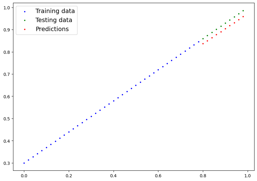
# Final values after 100 epochs
y_final = model(X_test).detach().numpy()
 
 
plot_predictions(predictions=y_final)

Output:

<Figure size 1000x700 with 1 Axes>

plt.plot(range(epochs), train_loss_per_epoch, label="Train Loss")
plt.plot(range(0, epochs, 10), test_loss_per_interval, label="Test Loss")
plt.title("Training and Testing Loss Curves")
plt.xlabel("Epochs")
plt.ylabel("MSE Loss")
plt.legend()

Output:

<matplotlib.legend.Legend at 0x771b96c473b0>

Output:

<Figure size 640x480 with 1 Axes>

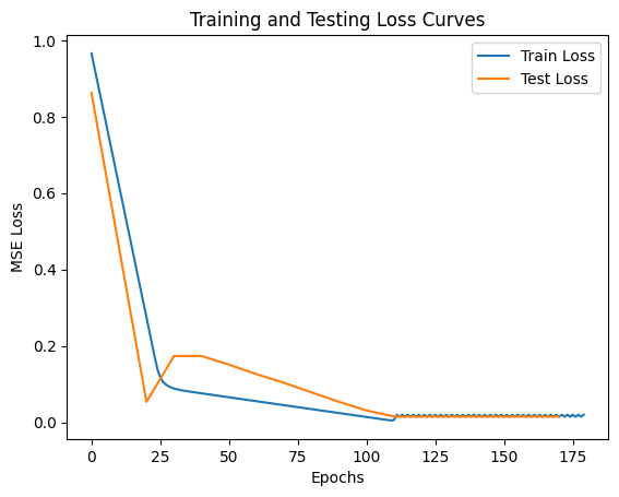
There’s an interesting inflection point happening here, which potentially tells me that the model hit a local optimum. This makes sense since the initial different in value between the initial guess and the actual value was quite large (like we were off by 100%).

It could imply that the learning rate is too high as we basically end up overshooting. Or actually because the train set is biased towards lower numbers, causing it to overshoot.

model.state_dict() # comparing to a weight of 0.7 and bias of 0.3

Output:

OrderedDict([('weights', tensor([0.6791])), ('bias', tensor([0.2933]))])

Saving and Loading Model

Now that model has been trained, maybe we wanna save the weights we got to (more important when the model is larger, large to the point where it holds value because of its lack of ease of reproducibility). Note, model here refers to like more than just the weights. GENERALLY WE SAVE THE STATE DICT OF THE MODEL. Its safer than saving the entire model, objects and all, as refactors can cause it to break really badly.

torch.save saves the model as a serialized pickle file.
torch.load unpickles the model and loads the python object files into memory

from pathlib import Path
 
# create path to directory
MODEL_PATH = Path("models")
MODEL_PATH.mkdir(parents=True, exist_ok=True)
 
# create model filename
MODEL_NAME = "01_workflow_model_0.pth"
MODEL_SAVE_PATH = MODEL_PATH/MODEL_NAME
 
# save the model
torch.save(obj=model.state_dict(), f=MODEL_SAVE_PATH)
 
!ls -l models/01_workflow_model_0.pth

Output:

-rw-rw-r-- 1 eddy eddy 1989 Oct 24 11:03 models/01_workflow_model_0.pth

new_model = LinearRegressionModel()
 
# load the model
new_model.load_state_dict(torch.load(f=MODEL_SAVE_PATH))
new_model.state_dict()

Output:

OrderedDict([('weights', tensor([0.6791])), ('bias', tensor([0.2933]))])

Put it all in CUDA

Just need to be more explicit with devices

import torch
from torch import nn
import matplotlib.pyplot as plt
 
torch.__version__
 
device = "cuda" if torch.cuda.is_available() else "cpu"
print(device)
 
# create some data
weight = 1.1
bias = -0.4
 
start = 0
stop = 100
step = 2
X = torch.arange(start, stop, step, device=device)
y = weight * X + bias
 
split = int(0.8 * len(X))
X_train, X_test = X[:split], X[split:]
y_train, y_test = y[:split], y[split:]
 
# Model, Loss, Optimizer Constructs
class LinearRegressionModelCUDA(nn.Module):
  def __init__(self, device=None):
    super().__init__()
 
    self.weight = nn.Parameter(torch.randn(1, dtype=torch.float, device=device), requires_grad=True)
    self.bias = nn.Parameter(torch.randn(1, dtype=torch.float, device=device), requires_grad=True)
 
  def forward(self, x : torch.Tensor) -> torch.Tensor:
    return self.weight * x + self.bias
 
model_cuda = LinearRegressionModelCUDA(device=device)
loss_fn = torch.nn.L1Loss()
optimizer = torch.optim.SGD(model_cuda.parameters(), lr=0.01)
 
# ------------------------------------------------------------------------------------
# There are smaller ways to handle GPU, one is to build on CPU first and then load onto GPU
# The downside of this is that if the model is large, it will fill up your RAM.
model_cpu = LinearRegressionModel()
model_cpu_then_cuda = model_cpu.to(device=device)
print(f"moving to cuda model state dict: {model_cpu_then_cuda.state_dict()}")
 
# Another way is to use context manager
with torch.device(device):
  model_context_cuda = LinearRegressionModel()
  print(f"moving to cuda model state dict: {model_context_cuda.state_dict()}")
 
# Another way is to set the global default device to GPU, but we lose control
# torch.set_default_device(device)
 
# The way I wrote it above feels better for the sake of control, either use my way or the context manager
# ------------------------------------------------------------------------------------
 
# begin train test loop
epochs = 200
 
cuda_train_loss_epoch = []
cuda_test_loss_epoch = []
 
for e in range(epochs):
  model_cuda.train()
 
  y_pred = model_cuda(X_train)
 
  train_loss = loss_fn(y_pred, y_train)
 
  cuda_train_loss_epoch.append(train_loss.cpu().detach().numpy())
 
  optimizer.zero_grad()
 
  train_loss.backward()
 
  optimizer.step()
 
  if (e%10 == 0):
    model_cuda.eval()
    
    with torch.inference_mode():
      y_pred = model_cuda(X_test)
      test_loss = loss_fn(y_pred, y_test)
 
      cuda_test_loss_epoch.append(test_loss.cpu().detach().numpy())
      print(f"Epoch {e} | MSE LOSS TRAIN {train_loss} | MSE TEST LOSS {test_loss}")
 
print("complete")
 
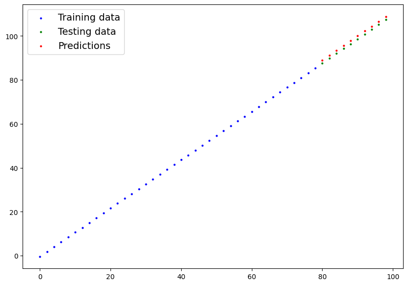
y_final = model_cuda(X_test).cpu().detach().numpy()
 
plot_predictions(train_data=X_train.cpu(), train_labels=y_train.cpu(), test_data=X_test.cpu(), test_labels=y_test.cpu(), predictions=y_final)

Output:

cuda
moving to cuda model state dict: OrderedDict({'weights': tensor([-1.7939], device='cuda:0'), 'bias': tensor([-1.0151], device='cuda:0')})
moving to cuda model state dict: OrderedDict({'weights': tensor([2.3062], device='cuda:0'), 'bias': tensor([-0.5731], device='cuda:0')})
Epoch 0 | MSE LOSS TRAIN 52.44105911254883 | MSE TEST LOSS 86.501953125
Epoch 10 | MSE LOSS TRAIN 7.6377272605896 | MSE TEST LOSS 19.028940200805664
Epoch 20 | MSE LOSS TRAIN 7.045223236083984 | MSE TEST LOSS 20.371456146240234
Epoch 30 | MSE LOSS TRAIN 6.452719211578369 | MSE TEST LOSS 21.713964462280273
Epoch 40 | MSE LOSS TRAIN 5.860215663909912 | MSE TEST LOSS 23.056476593017578
Epoch 50 | MSE LOSS TRAIN 5.267711639404297 | MSE TEST LOSS 24.398983001708984
Epoch 60 | MSE LOSS TRAIN 4.675207614898682 | MSE TEST LOSS 25.741491317749023
Epoch 70 | MSE LOSS TRAIN 4.082703590393066 | MSE TEST LOSS 27.084003448486328
Epoch 80 | MSE LOSS TRAIN 3.7257111072540283 | MSE TEST LOSS 27.890981674194336
Epoch 90 | MSE LOSS TRAIN 3.525723695755005 | MSE TEST LOSS 28.34095573425293
Epoch 100 | MSE LOSS TRAIN 3.325739622116089 | MSE TEST LOSS 28.790918350219727
Epoch 110 | MSE LOSS TRAIN 3.1257519721984863 | MSE TEST LOSS 29.24088478088379
Epoch 120 | MSE LOSS TRAIN 2.925766706466675 | MSE TEST LOSS 29.69085693359375
Epoch 130 | MSE LOSS TRAIN 2.7257823944091797 | MSE TEST LOSS 30.140823364257812
Epoch 140 | MSE LOSS TRAIN 2.5257949829101562 | MSE TEST LOSS 30.590789794921875
Epoch 150 | MSE LOSS TRAIN 2.3258092403411865 | MSE TEST LOSS 31.040760040283203
Epoch 160 | MSE LOSS TRAIN 2.125824213027954 | MSE TEST LOSS 31.49072265625
Epoch 170 | MSE LOSS TRAIN 1.925837516784668 | MSE TEST LOSS 31.940692901611328
Epoch 180 | MSE LOSS TRAIN 1.725852370262146 | MSE TEST LOSS 32.390663146972656
Epoch 190 | MSE LOSS TRAIN 1.5258668661117554 | MSE TEST LOSS 32.840633392333984
complete

Output:

<Figure size 1000x700 with 1 Axes>

Building with Pytorch Linear Model

You can define nn.Parameter to derive basically any model architecture through first principles, but luckily PyTorch provides some pre-implemented layers to make things easier.

class LinearRegressionModelLayers(nn.Module):
  def __init__(self, device=None):
    super().__init__()
 
    self.linear_layer = nn.Linear(in_features=1, out_features=1, device=device)
  
  def forward(self, x: torch.Tensor) -> torch.Tensor:
    return self.linear_layer(x)
  
with torch.device(device):
  model_v2 = LinearRegressionModelLayers()
  print(model_v2.state_dict())

Output:

OrderedDict({'linear_layer.weight': tensor([[-0.1725]], device='cuda:0'), 'linear_layer.bias': tensor([0.1621], device='cuda:0')})

import pathlib as Path
 
MODEL_NAME = "01_workflow_model_cuda_1.pth"
MODEL_SAVE_PATH = MODEL_PATH / MODEL_NAME
 
torch.save(model_v2.state_dict(), f=MODEL_SAVE_PATH)
 
!ls -l models/01_workflow_model_cuda_1.pth

Output:

-rw-rw-r-- 1 eddy eddy 2157 Oct 24 11:05 models/01_workflow_model_cuda_1.pth

load_cuda_model = LinearRegressionModelLayers()
 
load_cuda_model.load_state_dict(torch.load(MODEL_SAVE_PATH))
# .load_state_dict(torch.load(modelpath))
# .load_state_dict(torch.load(modelpath)) torch.load(model_path) .load_state_dict(torch.load(modelpath))
# model.load_state_dict(torch.load(model_path))
 
load_cuda_model.state_dict()

Output:

OrderedDict([('linear_layer.weight', tensor([[-0.1725]])),
             ('linear_layer.bias', tensor([0.1621]))])

Explorer

The PyTorch Workflow

PyTorch Workflow

PyTorch Model Workflow Essentials

Torch.nn

Loss Function and Optimizer

Time to train and test!

Saving and Loading Model

Put it all in CUDA

Building with Pytorch Linear Model

Graph View

Table of Contents