Kalman Filter

proprioception stateEstimation

A recursive algorithm used to estimate the state of a linear system based on noisy measurements.

Setup

There’s a ton of variables to keep track of:

• ${\mathbf{x}}_k\in {\mathbb{R}}^n$ is the state vector at time $k$
• ${\mathbf{F}}_k\in {\mathbb{R}}^{n\times n}$ is the state transition matrix, how state changes overtime on its own (irrespective of the input)
• ${\mathbf{B}}_k\in {\mathbb{R}}^{n\times m}$ is the control input matrix, maps control input to its effect on the state5
• ${\mathbf{u}}_k\in {\mathbb{R}}^m$ is the control input
• ${\mathbf{z}}_k\in {\mathbb{R}}^p$ is the measurement vector
• ${\mathbf{H}}_k\in {\mathbb{R}}^{p\times n}$ is the measurement matrix, maps the true state to what the sensor should measure (without noise)
• ${\mathbf{w}}_k\sim \mathcal{N}(0,{\mathbf{Q}}_k)$ is the process noise
• ${\mathbf{v}}_k\sim \mathcal{N}(0,{\mathbf{R}}_k)$ is the measurement noise

The goal of the Kalman Filter is to estimate a hidden state of a linear system from the noisy measurements that we get.

$${\mathbf{x}}_k={\mathbf{F}}_k{\mathbf{x}}_{k-1}+{\mathbf{B}}_k{\mathbf{u}}_k+{\mathbf{w}}_k$$

This is telling us how the hidden state of a linear system can be modeled as a function of how the linear system evolves without control input + how the system evolves with control input + process noise.

$${\mathbf{z}}_k={\mathbf{H}}_k{\mathbf{x}}_k+{\mathbf{v}}_k$$

This is telling us how the measurement of our states is modeled as a function of our hidden state mapped to our sensor measurements + some measurement noise.

Hidden state refers to the "underlying" state of the system. It is the true state of the system. We never have a direct understanding of this state in real life, we only have noisey measurements that get us there.

Two-steps

Because we will never know the true hidden state ${\mathbf{x}}_k$, we are stuck with making our best guess ${\hat{\mathbf{x}}}_k$. The Kalman filter is just a way to try to get a nice $\hat{\mathbf{x}}$.

A Kalmann Filter has two main steps:

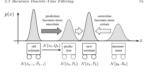
Predict Step

First we predict the current hidden state, and its covariance from the previous state and its covariance. These are priors they arent the final form of ${\hat{\mathbf{x}}}_{k|k}$ and its covariance ${\mathbf{P}}_{k|k}$

$${\hat{\mathbf{x}}}_{k|k-1}={\mathbf{F}}_k{\hat{\mathbf{x}}}_{k-1|k-1}+{\mathbf{B}}_k{\mathbf{u}}_k$$

This is telling us that to compute the state prior, we take the sum of how the system evolves naturally without the control input (called the state transition matrix) and how the state evolves with the control input.

$${\mathbf{P}}_{k|k-1}={\mathbf{F}}_k{\mathbf{P}}_{k-1|k-1}{\mathbf{F}}_k^T+{\mathbf{Q}}_k$$

This is telling us that to compute the state covariance prior, we take the product of the previous state covariance and the state transition matrix squared, then sum it with the covariance of our process noise.

Update Step

Here we take into account our measurements and try to reconciliate them with our predicted state and state covariance priors.

We first compute something called the Kalman Gain

$${\mathbf{K}}_k=\frac{{\mathbf{P}}_{k|k-1}{\mathbf{H}}_k^T}{({\mathbf{H}}_k{\mathbf{P}}_{k|k-1}{\mathbf{H}}_k^T+{\mathbf{R}}_k)}$$

The Kalman Gain tells us how much we trust our prediction over our trust in our measurement.

We use the computed Kalman gain to do a final update on our state and covariance

$${\hat{\mathbf{x}}}_{k|k}={\hat{\mathbf{x}}}_{k|k-1}+{\mathbf{K}}_k({\mathbf{z}}_k-{\mathbf{H}}_k{\hat{\mathbf{x}}}_{k|k-1})$$

This is telling us that the updated state is given by the predicted state plus the error between our real measurement and our measurement should we have gotten it from our prior, multiplied by the Kalman Gain

We also use the Kalman Gain to update the state covariance

$${\mathbf{P}}_{k|k}=(\mathbf{I}-{\mathbf{K}}_k{\mathbf{H}}_k){\mathbf{P}}_{k|k-1}$$

This is telling us that the updated state covariance (our certainty in the state estimate), is given by our confidence in the measurement. If confidence is high, state covariance goes to 0. If its low, state covariance remains as the prior covariance we computed (which could bloat)

---

EXAMPLE (FULL CONFIDENCE IN MEASUREMENT) Kalman Gain is interesting, intuitively, if we assume that our measurement noise is tiny, then that means ${\mathbf{R}}_k\to 0$

$${\mathbf{K}}_k=\frac{{\mathbf{P}}_{k|k-1}{\mathbf{H}}_k^T}{({\mathbf{H}}_k{\mathbf{P}}_{k|k-1}{\mathbf{H}}_k^T+0)}={\mathbf{H}}_k^{-1}$$

Which, as you will see, tells our update step to completely trust the entire measurement (because its noise is 0).

If we assumed that our measurement is perfectly accurate, no noise. Then ${\mathbf{K}}_k={\mathbf{H}}_k^{-1}$

$${\hat{\mathbf{x}}}_{k|k}={\hat{\mathbf{x}}}_{k|k-1}+\underset{\text{convert back to state}}{\underbrace{{\mathbf{H}}_k^{-1}}}(\underset{\begin{array}{c}\text{error between}\\ \text{measurement and}\\ \text{supposed measurement}\end{array}}{\underbrace{{\mathbf{z}}_k-{\mathbf{H}}_k{\hat{\mathbf{x}}}_{k|k-1}}})$$

Which means that we are just correcting our prior by the error it had with our measurement. Essentially making the state derived from the measurement, the state of the system.

Likewise, for covariance.

$${\mathbf{P}}_{k|k}=(\mathbf{I}-{\mathbf{H}}_k{\mathbf{K}}_k){\mathbf{P}}_{k|k-1}=(\mathbf{I}-{\mathbf{H}}_k{\mathbf{H}}_k^{-1}){\mathbf{P}}_{k|k-1}=(\mathbf{I}-\mathbf{I}){\mathbf{P}}_{k|k-1}$$ $${\mathbf{P}}_{k|k}=0$$

What this is telling us is that when we are fully confident in our measurement, we end up with no state covariance (uncertainty) at all. And our final state estimate is just our measurement.

---

EXAMPLE (NO CONFIDENCE IN MEASUREMENT) Here, our Kalman Gain goes to 0.

$${\mathbf{K}}_k=\frac{{\mathbf{P}}_{k|k-1}{\mathbf{H}}_k^T}{({\mathbf{H}}_k{\mathbf{P}}_{k|k-1}{\mathbf{H}}_k^T+\infty )}=0$$

Lets see how this affects our update.

$${\hat{\mathbf{x}}}_{k|k}={\hat{\mathbf{x}}}_{k|k-1}+{\mathbf{K}}_k({\mathbf{z}}_k-{\mathbf{H}}_k{\hat{\mathbf{x}}}_{k|k-1})$$ $${\hat{\mathbf{x}}}_{k|k}={\hat{\mathbf{x}}}_{k|k-1}+\underset{\text{We just ignore entirely}}{\underbrace{0({\mathbf{z}}_k-{\mathbf{H}}_k{\hat{\mathbf{x}}}_{k|k-1})}}={\hat{\mathbf{x}}}_{k|k-1}$$

So our state measurement just becomes our predicted state.

$${\mathbf{P}}_{k|k}=(\mathbf{I}-{\mathbf{H}}_k{\mathbf{K}}_k){\mathbf{P}}_{k|k-1}=(\mathbf{I}-0){\mathbf{P}}_{k|k-1}={\mathbf{P}}_{k|k-1}$$ $${\mathbf{P}}_{k|k}={\mathbf{P}}_{k|k-1}$$

So if we have no confidence in our measurement, then we just take the predicted state and its covariance at face value.

Note:

$${\mathbf{P}}_{k|k-1}={\mathbf{F}}_k{\mathbf{P}}_{k-1|k-1}{\mathbf{F}}_k^T+{\mathbf{Q}}_k$$

If our process noise is non-zero, then ${\mathbf{P}}_k$ will continue to bloat. If our state transition matrix is non-zero, then ${\mathbf{P}}_k$ will continue to bloat.

This means that the uncertainty of a Kalman filter will continue to bloat from its state transition matrix and process noise until a measurement of high-enough certainty is obtained.

---

EXAMPLE (DECENT CONFIDENCE IN MEASUREMENT) Here, I’m just going to walk through the whole step so that I remember how to write this.

Predict Step:

$${\hat{\mathbf{x}}}_{k|k-1}={\mathbf{F}}_k{\hat{\mathbf{x}}}_{k-1|k-1}+{\mathbf{B}}_k{\mathbf{u}}_k$$ $${\mathbf{P}}_{k|k-1}={\mathbf{F}}_k{\mathbf{P}}_{k-1|k-1}{\mathbf{F}}_k^T+{\mathbf{Q}}_k$$

Update Step:

$$0<{\mathbf{K}}_k=\frac{{\mathbf{P}}_{k|k-1}{\mathbf{H}}_k^T}{{\mathbf{H}}_k{\mathbf{P}}_{k|k-1}{\mathbf{H}}_k^T+{\mathbf{R}}_k}<{\mathbf{H}}_k^{-1}$$ $${\mathbf{P}}_{k|k}=(\underset{\begin{array}{c}\text{Kalman Gain can}\\ \text{only range from}\\ \text{0 to }\mathbf{I}\end{array}}{\underbrace{\mathbf{I}-{\mathbf{H}}_k{\mathbf{K}}_k}}){\mathbf{P}}_{k|k-1}$$

The introduction of a measurement can only make this better. Even a really shit measurement of high uncertainty could help with our measurement (marginally)

$${\hat{\mathbf{x}}}_{k|k}={\hat{\mathbf{x}}}_{k|k-1}+{\mathbf{K}}_k({\mathbf{z}}_k-{\mathbf{H}}_k{\hat{\mathbf{x}}}_{k|k-1})$$

So this means that the Kalman gain directly affects how much we want our measurement to affect our state estimate. It can range from no effect at all (0), or full correction effect.

---

EXAMPLE (PROCESS NOISE) Process noise tells us how much we should trust the model, based on how noisy our environment can be. Higher process noise means that we will bloat our uncertainty faster the longer we wait for a new measurement.

Predict Step

$${\hat{\mathbf{x}}}_{k|k-1}={\mathbf{F}}_k{\hat{\mathbf{x}}}_{k-1|k-1}+{\mathbf{B}}_k{\mathbf{u}}_k$$ $${\mathbf{P}}_{k|k-1}={\mathbf{F}}_k{\mathbf{P}}_{k-1|k-1}{\mathbf{F}}_k^T+{\mathbf{Q}}_k={\mathbf{F}}_k{\mathbf{P}}_{k-1|k-1}{\mathbf{F}}_k^T+\infty =\infty$$

Update Step

$${\mathbf{K}}_k=\frac{{\mathbf{P}}_{k|k-1}{\mathbf{H}}_k^T}{{\mathbf{H}}_k{\mathbf{P}}_{k|k-1}{\mathbf{H}}_k^T+{\mathbf{R}}_k}=\frac{\infty }{\infty {\mathbf{H}}_k}={\mathbf{H}}_k^{-1}$$ $${\hat{x}}_{k|k}={\hat{\mathbf{x}}}_{k|k-1}+{\mathbf{K}}_k({\mathbf{z}}_k-{\mathbf{H}}_k{\hat{\mathbf{x}}}_{k|k-1})={\hat{\mathbf{x}}}_{k|k-1}+{\mathbf{H}}_k^{-1}({\mathbf{z}}_k-{\mathbf{H}}_k{\hat{\mathbf{x}}}_{k|k-1})$$ $${\mathbf{P}}_{k|k}=(\mathbf{I}-{\mathbf{H}}_k{\mathbf{K}}_k){\mathbf{P}}_{k|k-1}=\infty$$

If we have infinite process noise, then the whole system collapses lol.

The increase of process noise will result in our system become more uncertain faster. This means that we need more measurements to counteract the rate at which the state covariance is increasing.

worldModeling